Linear Regression

Overview

Linear regression is a fundamental supervised learning algorithm that models the relationship between a dependent variable (target) and one or more independent variables (features) by fitting a linear equation to the observed data.

Linear Regression

Linear Regression: Fitting a line to data points by minimizing the sum of squared residuals

Key concepts in linear regression:

  • Simple Linear Regression: One independent variable
  • Multiple Linear Regression: Multiple independent variables
  • Polynomial Regression: Non-linear relationships using polynomial features
  • Regularization: Ridge (L2), Lasso (L1), and Elastic Net

Core Concepts

  • The Linear Model

    The linear regression model can be expressed as:

    y = β₀ + β₁x₁ + β₂x₂ + ... + βₙxₙ + ε

    Where:

    • y is the dependent variable (target)
    • x₁, x₂, ..., xₙ are independent variables (features)
    • β₀ is the intercept (bias term)
    • β₁, β₂, ..., βₙ are coefficients (weights)
    • ε is the error term
  • Loss Function and Optimization

    Linear regression typically uses Mean Squared Error (MSE) as the loss function:

    MSE = (1/n) Σ(y_true - y_pred)²

    The goal is to find the coefficients that minimize this loss function. This can be done through:

    • Normal Equation: Direct analytical solution
    • Gradient Descent: Iterative optimization
  • Regularization Techniques

    Regularization helps prevent overfitting by adding a penalty term to the loss function:

    • Ridge Regression (L2): Adds squared magnitude of coefficients
    • Lasso Regression (L1): Adds absolute value of coefficients
    • Elastic Net: Combines both L1 and L2 regularization
  • Residual Analysis

    Key aspects of residual analysis:

    • Residual plots to check linearity assumption
    • Q-Q plots to check normality of residuals
    • Scale-location plots to check homoscedasticity
    • Leverage plots to identify influential points
  • Cross-Validation

    Methods for model validation:

    • K-fold cross-validation
    • Leave-one-out cross-validation
    • Time series cross-validation
  • Feature Selection

    Techniques for selecting relevant features:

    • Forward selection
    • Backward elimination
    • Stepwise selection
    • Lasso regularization

Implementation

  • Comprehensive Linear Regression Examples

    Implementation of various linear regression techniques with visualization and analysis.
    
    import numpy as np
    import pandas as pd
    import matplotlib.pyplot as plt
    from sklearn.linear_model import LinearRegression, Ridge, Lasso, ElasticNet
    from sklearn.preprocessing import PolynomialFeatures, StandardScaler
    from sklearn.model_selection import train_test_split, cross_val_score
    from sklearn.metrics import mean_squared_error, r2_score
    from sklearn.pipeline import Pipeline
    
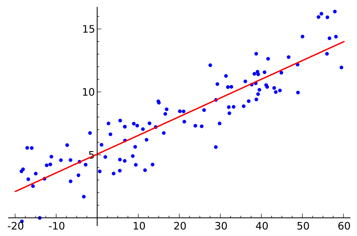
    # --- 1. Simple Linear Regression ---
    def simple_linear_regression_example():
        # Generate synthetic data
        np.random.seed(42)
        X = 2 * np.random.rand(100, 1)
        y = 4 + 3 * X + np.random.randn(100, 1) * 0.5
    
        # Split the data
        X_train, X_test, y_train, y_test = train_test_split(X, y, test_size=0.2, random_state=42)
    
        # Create and train the model
        model = LinearRegression()
        model.fit(X_train, y_train)
    
        # Make predictions
        y_pred = model.predict(X_test)
    
        # Print results
        print("Simple Linear Regression Results:")
        print(f"Coefficient: {model.coef_[0][0]:.4f}")
        print(f"Intercept: {model.intercept_[0]:.4f}")
        print(f"R² Score: {r2_score(y_test, y_pred):.4f}")
    
        # Visualize results
        plt.figure(figsize=(10, 6))
        plt.scatter(X_train, y_train, color='blue', label='Training Data')
        plt.scatter(X_test, y_test, color='green', label='Test Data')
        plt.plot(X_test, y_pred, color='red', label='Predictions')
        plt.xlabel('X')
        plt.ylabel('y')
        plt.title('Simple Linear Regression')
        plt.legend()
        plt.grid(True)
        # plt.show()
    
    # --- 2. Multiple Linear Regression ---
    def multiple_linear_regression_example():
        # Generate synthetic data
        np.random.seed(42)
        X = np.random.rand(100, 3)  # 3 features
        y = 4 + 2*X[:, 0] + 3*X[:, 1] - 1*X[:, 2] + np.random.randn(100) * 0.5
    
        # Split and scale the data
        X_train, X_test, y_train, y_test = train_test_split(X, y, test_size=0.2, random_state=42)
        
        scaler = StandardScaler()
        X_train_scaled = scaler.fit_transform(X_train)
        X_test_scaled = scaler.transform(X_test)
    
        # Create and train the model
        model = LinearRegression()
        model.fit(X_train_scaled, y_train)
    
        # Make predictions
        y_pred = model.predict(X_test_scaled)
    
        # Print results
        print("
    Multiple Linear Regression Results:")
        for i, coef in enumerate(model.coef_):
            print(f"Coefficient {i+1}: {coef:.4f}")
        print(f"Intercept: {model.intercept_:.4f}")
        print(f"R² Score: {r2_score(y_test, y_pred):.4f}")
    
    # --- 3. Polynomial Regression ---
    def polynomial_regression_example():
        # Generate synthetic data with non-linear relationship
        np.random.seed(42)
        X = np.linspace(-3, 3, 100).reshape(-1, 1)
        y = 0.5 * X**2 + X + 2 + np.random.randn(100, 1) * 0.5
    
        # Split the data
        X_train, X_test, y_train, y_test = train_test_split(X, y, test_size=0.2, random_state=42)
    
        # Create polynomial features
        degrees = [1, 2, 3]  # Try different polynomial degrees
        plt.figure(figsize=(15, 5))
    
        for i, degree in enumerate(degrees, 1):
            # Create polynomial pipeline
            model = Pipeline([
                ('poly', PolynomialFeatures(degree=degree)),
                ('linear', LinearRegression())
            ])
    
            # Fit the model
            model.fit(X_train, y_train)
            y_pred = model.predict(X_test)
    
            # Plot results
            plt.subplot(1, 3, i)
            plt.scatter(X_train, y_train, color='blue', label='Training Data', alpha=0.5)
            plt.scatter(X_test, y_test, color='green', label='Test Data', alpha=0.5)
            
            # Sort X for smooth curve plotting
            X_sort = np.sort(X, axis=0)
            y_curve = model.predict(X_sort)
            plt.plot(X_sort, y_curve, color='red', label=f'Degree {degree}')
            
            plt.xlabel('X')
            plt.ylabel('y')
            plt.title(f'Polynomial Regression (Degree {degree})')
            plt.legend()
            plt.grid(True)
    
        plt.tight_layout()
        # plt.show()
    
    # --- 4. Regularized Regression ---
    def regularized_regression_example():
        # Generate synthetic data with many features
        np.random.seed(42)
        n_samples, n_features = 100, 20
        X = np.random.randn(n_samples, n_features)
        # True coefficients: only first 5 features are relevant
        true_coef = np.zeros(n_features)
        true_coef[:5] = [2, -1, 1.5, -0.5, 1]
        y = np.dot(X, true_coef) + np.random.randn(n_samples) * 0.1
    
        # Split and scale the data
        X_train, X_test, y_train, y_test = train_test_split(X, y, test_size=0.2, random_state=42)
        scaler = StandardScaler()
        X_train_scaled = scaler.fit_transform(X_train)
        X_test_scaled = scaler.transform(X_test)
    
        # Define models with different regularization
        models = {
            'Linear': LinearRegression(),
            'Ridge': Ridge(alpha=1.0),
            'Lasso': Lasso(alpha=1.0),
            'ElasticNet': ElasticNet(alpha=1.0, l1_ratio=0.5)
        }
    
        # Train and evaluate each model
        print("
    Regularized Regression Results:")
        for name, model in models.items():
            model.fit(X_train_scaled, y_train)
            y_pred = model.predict(X_test_scaled)
            mse = mean_squared_error(y_test, y_pred)
            r2 = r2_score(y_test, y_pred)
            print(f"
    {name} Regression:")
            print(f"MSE: {mse:.4f}")
            print(f"R² Score: {r2:.4f}")
            print(f"Number of non-zero coefficients: {np.sum(np.abs(model.coef_) > 1e-10)}")
    
        # Visualize coefficients
        plt.figure(figsize=(12, 6))
        x = np.arange(n_features)
        width = 0.15
        
        for i, (name, model) in enumerate(models.items()):
            plt.bar(x + i*width, model.coef_, width, label=name, alpha=0.7)
        
        plt.xlabel('Feature Index')
        plt.ylabel('Coefficient Value')
        plt.title('Comparison of Coefficients Across Different Regularization Methods')
        plt.legend()
        plt.grid(True)
        # plt.show()
    
    # --- Main Execution ---
    if __name__ == "__main__":
        print("Running Linear Regression Examples...")
        
        # Run all examples
        simple_linear_regression_example()
        multiple_linear_regression_example()
        polynomial_regression_example()
        regularized_regression_example()
    
  • Linear Regression with scikit-learn

    Train a linear regression model using scikit-learn.

    from sklearn.linear_model import LinearRegression
    from sklearn.datasets import make_regression
    
    X, y = make_regression(n_samples=100, n_features=1, noise=10)
    model = LinearRegression()
    model.fit(X, y)
    print('Coefficient:', model.coef_)
    print('Intercept:', model.intercept_)
    
  • Linear Regression from Scratch (NumPy)

    Implement linear regression using the normal equation in NumPy.

    import numpy as np
    
    # Generate synthetic data
    np.random.seed(0)
    X = 2 * np.random.rand(100, 1)
    y = 4 + 3 * X + np.random.randn(100, 1)
    
    # Add bias term
    X_b = np.c_[np.ones((100, 1)), X]
    
    # Normal equation
    theta_best = np.linalg.inv(X_b.T.dot(X_b)).dot(X_b.T).dot(y)
    print('Intercept:', theta_best[0, 0])
    print('Slope:', theta_best[1, 0])
    

Interview Examples

Explain the assumptions of linear regression

What are the key assumptions of linear regression and how can they be verified?

Compare different types of regularization

Explain the differences between Ridge, Lasso, and Elastic Net regularization

Practice Questions

1. Derive the normal equation for linear regression Medium

Hint: Think about minimizing the sum of squared errors
\hat{\beta} = (X^TX)^{-1}X^Ty

2. Explain the difference between L1 and L2 regularization Easy

Hint: Consider their effects on the model parameters and feature selection

3. Implement linear regression with gradient descent Medium

Hint: Remember to compute the gradient of the cost function
import numpy as np def gradient_descent(X, y, learning_rate=0.01, iterations=1000): m = len(y) theta = np.zeros(X.shape[1]) cost_history = [] for i in range(iterations): prediction = np.dot(X, theta) error = prediction - y cost = (1/(2*m)) * np.sum(error**2) cost_history.append(cost) # Update theta theta = theta - (learning_rate/m) * np.dot(X.T, error) return theta, cost_history